Motivation
Experiencing binary search was like a divine revelation of the ingenuity of algorithms. How can computer code be so clever and efficient at the same time? We don’t thank the inventors enough 😏.
Among the great, simple, and everyday algorithms used is merge sort. It is a divide-and-conquer algorithm that works by taking a big problem, chunking it down into the smallest possible units, solving them, and adding up the results together. Read more about it here.
While deeply studying merge sort, a question I further asked after noticing its patterns is: Is this under the hood another binary search algorithm?
The beautiful binary search
Searching is fundamental to human existence, we are always asking the what, why, where, who, and when questions. This has resulted in most of our inventions, computers being one of their greatest. So, given an array of five items [4,5,1,2,4], how can you get an item from the list?
An easy approach would be to go through each item, compare them to 1, and return to the position where it was found. This approach is called linear search, which has been implemented here. This raises a question: what happens when the list is large enough, for example, your WhatsApp contact list? Searching through these items in linear time can be fast for 10 10-item lists; when the list becomes sufficiently large, the time it takes will frustrate any human.
What if the list is sorted ([1,2,3,4,5]), and we need to get the item at position 4 from the list? We have to change our thinking model. Going through each of these items linearly is lavishing time! Which introduces the binary search algorithm.
We can split the items into two arrays, [1,2] and [3,4,5], determine where the item we are searching for can be(left or right), discard the left array, and divide the right array into two [3], [4,5]. We discard the left array again and divide the right array into two [4] and [5]; the target is the only item in the right array. Notice it took us three divisions, two extra variables to store the separate arrays, and two decision statements - Is the item on the left or the right? Is the item the only item in the array?
| |
We can use the above procedure to find out if the item is on the list. What if we need the index where the item is?
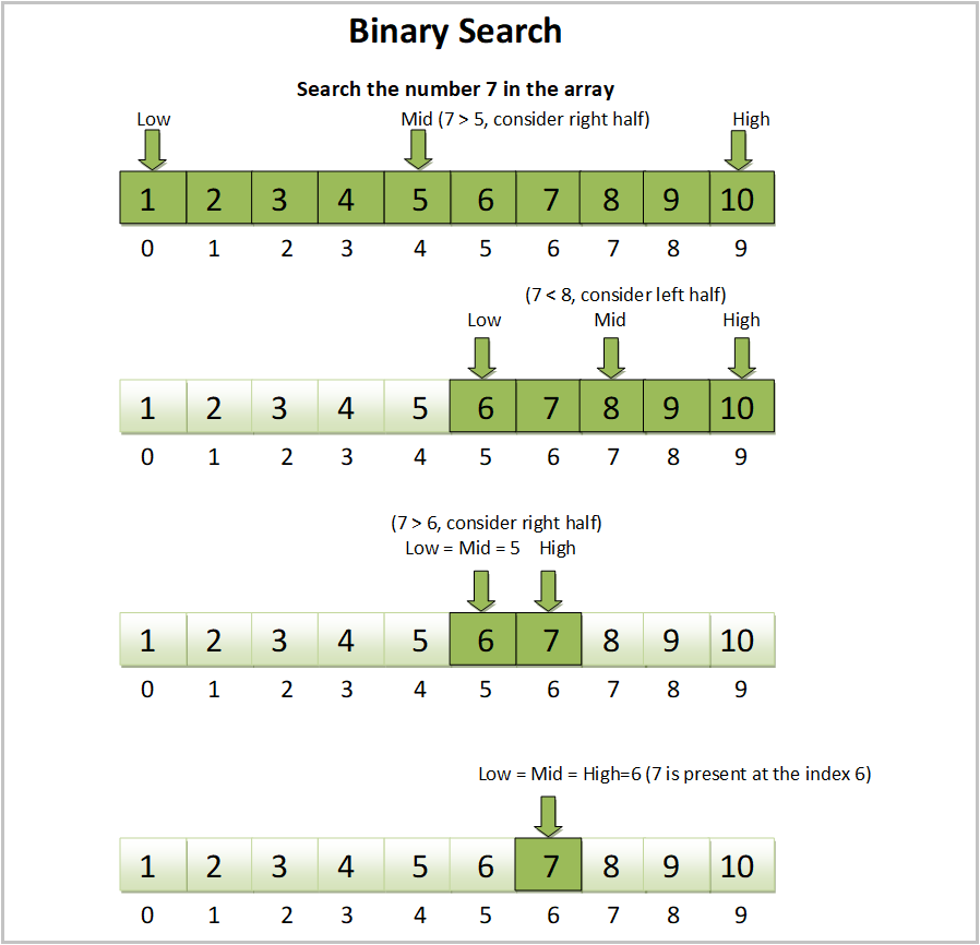
Recall our sorted array of 5 items [1,2,3,4,5]. Instead of dividing, we can have two variables: start point and end point. The start point of the array is 0, the endpoint is the length of the array -1 - in our case 4, and finally, keep a midpoint (floor division of the length of the array).
Then, we can check if the target is equal to the value of the midpoint. If yes, we return the index of the midpoint; if no, we check if the item is greater than the midpoint, if it is, then we set the value of the left handle to be the midpoint, if it is not, we set the value of the right handle to be the midpoint and this is to discard half of the items in the list, either from the left till the midpoint or from the midpoint to the right.
We do these steps up until we find a midpoint where the value is the same as the target.
For the most binary search, it could be written with a loop, but it is cleaner to implement it as a recursive algorithm - this is proving the statement that nearly all recursive algorithms can be implemented with a loop.
| |
The iterative implementation explicitly expresses the formal definition and internal operation of a binary search algorithm,
Is the midpoint element the target?
Yes, return it.
No, then,
Adjust the left or right handles and check the midpoint again.
Sweet!
Merge Sorting
Faced with the challenge of sorting the list [4,5,1,2,4] in ascending order, as we did for searching, we could pick one item at a time and insert it into its exact position. We could achieve this using the insertion sort algorithm:
| |
Insertion sort runs in O(n^2), but with a divide and conquer algorithm, we can run in O(nlgn) time.
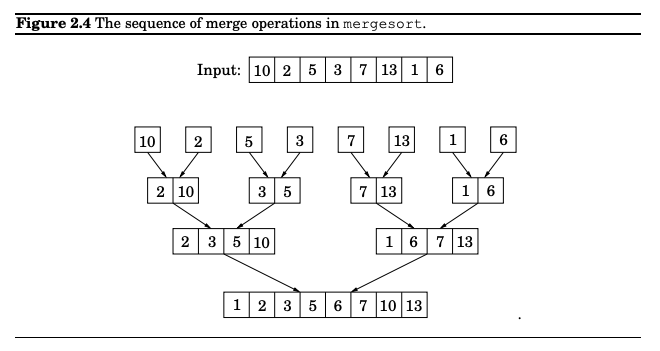
Merge sort is another divide and conquer algorithm that works just like any other would. It takes an input array, breaks it into chunks of smaller subarrays, sorts the subarrays, and merges the results, all these in O(nlgn) time.
Sorting the list of numbers, instead of taking an item and inserting it in place of another, we rather tear apart the entire list and rebuild a new one with the right order. Starting with [4,5,3,2,1], we can split it into [4,5] and [3,2,1]. And again, we can split these into [4] and [5] for the left, and also [3] and [2, 1] for the right. Lastly [2] and [1]. So far, the breakdown looks like this:
We begin from the last item row, sort the items, and then merge them in place and up to the top row:
In implementation, the code looks like this:
| |
This works by splitting the array into two until there is only one item remaining in the final array. Then it walks back up, bringing the items in the left and right arrays to compare their first items to identify which comes first to insert it into the position in the main array.
When one of the sub-arrays is empty - nothing left to sort - it spreads the remnant in the nonempty subarray to the right of the main array. Hence, the left items are always sorted after each merge procedure call.
The meat of merge sort is in the merge procedure, but regardless of the subtleties, the importance of the merge_sort procedure can not be ignored. A closer look reveals a resemblance to its counterpart divide and conquer algorithms, in our case, the binary search!

Like Binary Search Like Merge Sort
The question I often get with merge sort and other divide-and-conquer algorithms is: How does this work?
The problem is not understanding merge sort, it is in understanding divide and conquer algorithms.
The goal of a divide-and-conquer algorithm is to break a problem into the smallest unit of subproblems that can be solved easily. Not just for sorting or using binary search to find an element’s index in a list. We can use it for other problems like the below:
When conceptualizing a problem, the first insight is understanding if the solution to the problem can be determined in a single execution statement and if the problem input can be split into smaller versions such that a single split is a subset of the actual input such that we could solve it easily.
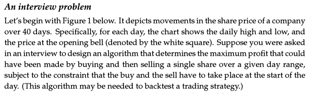
In the above example, although two values are required - entry and exit values- note that the lowest buy price will always be on the left, and the highest sell price will be on the right. If you have the array [[10, 12], [12, 11.5], [11.5, 13],[13, 9.01]], when you buy at 10 from the first item in the list and sell at 13.00 in the last index. A brute-force solution should run in O(n^2).
However, the best solution will continuously split the array into halves(the divide stage), up until there is one array left, and track the optimum buy price from the left array and the optimum sell price in the right array. This takes into consideration the intricacies of empty an array, an array with one element, and an extra edge case unique to this problem, when the price decreases monotonically - then there is no way to determine a selling price.
Notice that I have referenced a problem that uses divide and conquer to solve a problem that seems different from merge sort and binary search; it is expecting us to pick(which might sound like a search problem) two best items from a list.
What you should know
When these questions arise, it is as a result of an incomplete understanding of fundamental concepts.
While our jobs might require us to sort a list or search for an item in a sorted list – knowing merge sort will suffice – real-life problems do not present themselves in this fashion, as demonstrated.
When solving a problem, the default is to look for a brute-force solution that performs in the worst possible time but satisfies the definition of an algorithm. To get the best possible performance out of the algorithm, the saving grace is understanding the fundamental concepts and being able to relate a problem to one of them.
So, always choose to understand the fundamentals rather than example use cases of a fundamental concept. After that, merge sort, binary search, and other seemingly hard algorithms will present themselves, like the sun in the day!